
Data validation is a critical process in computing and data management that ensures data accuracy, consistency, and quality before it is used or processed. Data validation is fundamental to maintaining high-quality data that supports accurate insights.
Drop-down lists are a powerful data validation feature in Excel that helps control and standardize data entry.
Let’s look at how we can create them (Drop down list).

Recognize the image above? It is our conditional formatting dashboard from Day 1 of the #excelin60days challenge.
We could achieve data validation through list in excel; these three ways are centered on the presentation of the data for the list, much like the list library.
Method 1
The first method is you inputting the values of your list separated by comma. Let’s do it..
Highlight the cells you want to apply the drop down. In our example we will be highlighting the Category column. Ensure you highlight only the area you want to enter data and not your headings.
Go to Data on the Excel menu Ribbon

Then click on Data Validation under Data Tools Group. Once you do, the Data Validation settings will pop up.

Under allow, you will currently see Any value (this indicates that excel will currently accept any value entered into the spreadsheet)
Click the drop down to select List

In the source space enter the items under the category column separated by comma. Example: Food, Rent, Utilities, Transport, Entertainment, Healthcare
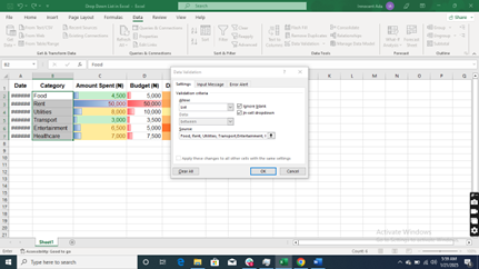
Then click OK

You will see a drop-down icon by the side of the Category Column. Click it to select the item of choice.
Method 2
Method 2 requires that you had a list repository somewhere in your sheet. That is to say you have your list items listed in one corner of your active sheet.
So, we will be using all the steps of the method one except we input the range of our list repository in the Source.
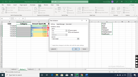
Then go ahead and click OK
Method 3
The third method requires that you have your list in a separate sheet. So, you enter the sheet address and repository range in the Source.
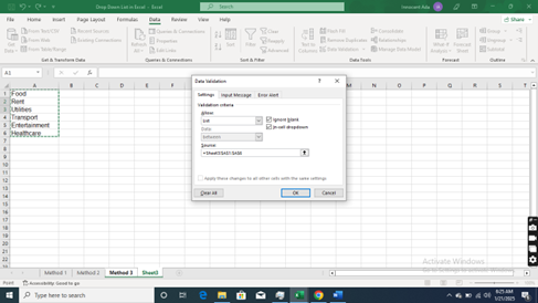
Then click OK

